From Modern 'Neural Network' to the Era of 'Deep Learning'

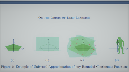
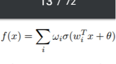
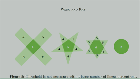
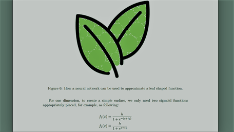
​In this section, we will introduce some important properties of neural networks. These properties partially explain the popularity neural network gains these days and also motivate the necessity of exploring deeper architecture. To be specific, we will discuss a set of universal approximation properties, in which each property has its condition. Then, we will show that although a shallow neural network is an universal approximator, deeper architecture can significantly reduce the requirement of resources while retaining the representation power. At last, we will also show some interesting properties discovered in the 1990s about backpropagation, which may inspire some related research today. 

​1.Universal Approximation Property

The step from perceptrons to basic neural networks is only placing the perceptrons together. By placing the perceptrons side by side, we get a single one-layer neural network and by stacking one one-layer neural network upon the other, we get a multi-layer neural network, which is often known as multi-layer perceptrons (MLP) (Kawaguchi, 2000).
​
One remarkable property of neural networks, widely known as universal approximation property, roughly describes that an MLP can represent any functions. Here we discussed this property in three different aspects: 

​• Boolean Approximation: an MLP of one hidden layer1 can represent any boolean function exactly.

​• Continuous Approximation: an MLP of one hidden layer can approximate any bounded continuous function with arbitrary accuracy.

​• Arbitrary Approximation: an MLP of two hidden layers can approximate any function with arbitrary accuracy.

​We will discuss these three properties in detail in the following paragraphs. To suit different readers’ interest, we will first offer an intuitive explanation of these properties and then offer the proofs. 

​1.1 Representation of any Boolean Functions 

​This approximation property is very straightforward. In the previous section we have shown that every linear preceptron can perform either AND or OR. According to De Morgan’s laws, every propositional formula can be converted into an equivalent Conjunctive Normal Form, which is an OR of multiple AND functions. Therefore, we simply rewrite the target Boolean function into an OR of multiple AND operations. Then we design the network in such a way: the input layer performs all AND operations, and the hidden layer is simply an OR operation.

​The formal proof is not very different from this intuitive explanation, we skip it for simplicity.

1.2 Approximation of any Bounded Continuous Functions

​Continuing from the linear representation power of perceptron discussed previously, if we want to represent a more complex function, showed in Figure 4 (a), we can use a set of linear perceptrons, each of them describing a halfspace. One of these perceptrons is shown in Figure 4 (b), we will need five of these perceptrons. With these perceptrons, we can bound the target function out, as showed in Figure 4 (c). The numbers showed in Figure 4 (c) represent the number of subspaces described by perceptrons that fall into the corresponding region. As we can see, with an appropriate selection of the threshold (e.g. θ = 5 in Figure 4 (c)), we can bound the target function out. Therefore, we can describe any bounded continuous function with only one hidden layer; even it is a shape as complicated as Figure 4 (d).

​This property was first shown in (Cybenko, 1989) and (Hornik et al., 1989). To be specific, Cybenko (1989) showed that, if we have a function in the following form: 

f(x) is dense in the subspace of where it is in. In other words, for an arbitrary function g(x) in the same subspace as f(x), we have 

where e > 0. In Equation 3, σ denotes the activation function (a squashing function back then), wi denotes the weights for the input layer and ωi denotes the weights for the hidden layer.

​This conclusion was drawn with a proof by contradiction: With Hahn-Banach Theorem and Riesz Representation Theorem, the fact that the closure of f(x) is not all the subspace where f(x) is in contradicts the assumption that σ is an activation (squashing) function.

​Till today, this property has drawn thousands of citations. Unfortunately, many of the later works cite this property inappropriately (Castro et al., 2000) because Equation 3 is not the widely accepted form of a one-hidden-layer neural network because it does not deliver a thresholded/squashed output, but a linear output instead. Ten years later after this property was shown, Castro et al. (2000) concluded this story by showing that when the final output is squashed, this universal approximation property still holds.

Note that, this property was shown with the context that activation functions are squashing functions. By definition, a squashing function σ : R → [0, 1] is a non-decreasing function with the properties limx→∞ σ(x) = 1 and limx→−∞ σ(x) = 0. Many activation functions of recent deep learning research do not fall into this category. 

1.3 Approximation of Arbitrary Functions

Before we move on to explain this property, we need first to show a major property regarding combining linear perceptrons into neural networks. Figure 5 shows that as the number of linear perceptrons increases to bound the target function, the area outside the polygon with the sum close to the threshold shrinks. Following this trend, we can use a large number of perceptrons to bound a circle, and this can be achieved even without knowing the threshold because the area close to the threshold shrinks to nothing. What left outside the circle is, in fact, the area that sums to N / 2 , where N is the number of perceptrons used.

​Therefore, a neural network with one hidden layer can represent a circle with arbitrary diameter. Further, we introduce another hidden layer that is used to combine the outputs of many different circles. This newly added hidden layer is only used to perform OR operation. Figure 6 shows an example that when the extra hidden layer is used to merge the circles from the previous layer, the neural network can be used to approximate any function. The target function is not necessarily continuous. However, each circle requires a large number of neurons, consequently, the entire function requires even more.

​This property was showed in (Lapedes and Farber, 1988) and (Cybenko, 1988) respectively. Looking back at this property today, it is not arduous to build the connections between this property to Fourier series approximation, which, in informal words, states that every function curve can be decomposed into the sum of many simpler curves. With this linkage, to show this universal approximation property is to show that any one-hiddenlayer neural network can represent one simple surface, then the second hidden layer sums up these simple surfaces to approximate an arbitrary function. 

As we know, one hidden layer neural network simply performs a thresholded sum operation, therefore, the only step left is to show that the first hidden layer can represent a simple surface. To understand the “simple surface”, with linkage to Fourier transform, one can imagine one cycle of the sinusoid for the one-dimensional case or a “bump” of a plane in the two-dimensional case. 

​Then, with f1(x) + f2(x), we create a simple surface with height 2h from t1 ≤ x ≤ t2. This could be easily generalized to n-dimensional case, where we need 2n sigmoid functions (neurons) for each simple surface. Then for each simple surface that contributes to the final function, one neuron is added onto the second hidden layer. Therefore, despite the number of neurons need, one will never need a third hidden layer to approximate any function. 

​Similarly to how Gibbs phenomenon affects Fourier series approximation, this approximation cannot guarantee an exact representation.

The universal approximation properties showed a great potential of shallow neural networks at the price of exponentially many neurons at these layers. One followed-up question is that how to reduce the number of required neurons while maintaining the representation power. This question motivates people to proceed to deeper neural networks despite that shallow neural networks already have infinite modeling power. Another issue worth attention is that, although neural networks can approximate any functions, it is not trivial to find the set of parameters to explain the data. In the next two sections, we will discuss these two questions respectively. 

2. The Necessity of Depth

The universal approximation properties of shallow neural networks come at a price of exponentially many neurons and therefore are not realistic. The question about how to maintain this expressive power of the network while reducing the number of computation units has been asked for years. Intuitively, Bengio and Delalleau (2011) suggested that it is nature to pursue deeper networks because 1) human neural system is a deep architecture (as we will see examples in Section 5 about human visual cortex.) and 2) humans tend to represent concepts at one level of abstraction as the composition of concepts at lower levels. Nowadays, the solution is to build deeper architectures, which comes from a conclusion that states the representation power of a k layer neural network with polynomial many neurons need to be expressed with exponentially many neurons if a k − 1 layer structured is used. However, theoretically, this conclusion is still being completed. 

​This conclusion could trace back to three decades ago when Yao (1985) showed the limitations of shallow circuits functions. Hastad (1986) later showed this property with parity circuits: “there are functions computable in polynomial size and depth k but requires exponential size when depth is restricted to k − 1”. He showed this property mainly by the application of DeMorgan’s law, which states that any AND or ORs can be rewritten as OR of ANDs and vice versa. Therefore, he simplified a circuit where ANDs and ORs appear one after the other by rewriting one layer of ANDs into ORs and therefore merge this operation to its neighboring layer of ORs. By repeating this procedure, he was able to represent the same function with fewer layers, but more computations.

Moving from circuits to neural networks, Delalleau and Bengio (2011) compared deep and shallow sum-product neural networks. They showed that a function that could be expressed with O(n) neurons on a network of depth k required at least O(2 √ n ) and O((n − 1)k ) neurons on a two-layer neural network. 

Further, Bianchini and Scarselli (2014) extended this study to a general neural network with many major activation functions including tanh and sigmoid. They derived the conclusion with the concept of Betti numbers, and used this number to describe the representation power of neural networks. They showed that for a shallow network, the representation power can only grow polynomially with respect to the number of neurons, but for deep architecture, the representation can grow exponentially with respect to the number of neurons. They also related their conclusion to VC-dimension of neural networks, which is O(p 2 ) for tanh (Bartlett and Maass, 2003) where p is the number of parameters.

Recently, Eldan and Shamir (2015) presented a more thorough proof to show that depth of a neural network is exponentially more valuable than the width of a neural network, for a standard MLP with any popular activation functions. Their conclusion is drawn with only a few weak assumptions that constrain the activation functions to be mildly increasing, measurable, and able to allow shallow neural networks to approximate any univariate Lipschitz function. Finally, we have a well-grounded theory to support the fact that deeper network is preferred over shallow ones. However, in reality, many problems will arise if we keep increasing the layers. Among them, the increased difficulty of learning proper parameters is probably the most prominent one. Immediately in the next section, we will discuss the main drive of searching parameters for a neural network: Backpropagation. 

​3. Backpropagation and Its Properties

​Before we proceed, we need to clarify that the name backpropagation, originally, is not referring to an algorithm that is used to learn the parameters of a neural network, instead, it stands for a technique that can help efficiently compute the gradient of parameters when gradient descent algorithm is applied to learn parameters (Hecht-Nielsen, 1989). However, nowadays it is widely recognized as the term to refer gradient descent algorithm with such a technique.

Compared to a standard gradient descent, which updates all the parameters with respect to error, backpropagation first propagates the error term at output layer back to the layer at which parameters need to be updated, then uses standard gradient descent to update parameters with respect to the propagated error. Intuitively, the derivation of backpropagation is about organizing the terms when the gradient is expressed with the chain rule. The derivation is neat but skipped in this paper due to the extensive resources available (Werbos, 1990; Mitchell et al., 1997; LeCun et al., 2015). Instead, we will discuss two interesting and seemingly contradictory properties of backpropagation.

3.1 Backpropagation Finds Global Optimal for Linear Separable Data

​Gori and Tesi (1992) studied on the problem of local minima in backpropagation. Interestingly, when the society believes that neural networks or deep learning approaches are believed to suffer from local optimal, they proposed an architecture where global optimal is guaranteed. Only a few weak assumptions of the network are needed to reach global optimal, including 

​• Pyramidal Architecture: upper layers have fewer neurons

​• Weight matrices are full row rank

​• The number of input neurons cannot smaller than the classes/patterns of data. 

​However, their approaches may not be relevant anymore as they require the data to be linearly separable, under which condition that many other models can be applied. 

3.2 Backpropagation Fails for Linear Separable Data

​On the other hand, Brady et al. (1989) studied the situations when backpropagation fails on linearly separable data sets. He showed that there could be situations when the data is linearly separable, but a neural network learned with backpropagation cannot find that boundary. He also showed examples when this situation occurs.

​His illustrative examples only hold when the misclassified data samples are significantly less than correctly classified data samples, in other words, the misclassified data samples might be just outliers. Therefore, this interesting property, when viewed today, is arguably a desirable property of backpropagation as we typically expect a machine learning model to neglect outliers. Therefore, this finding has not attracted many attentions.

However, no matter whether the data is an outlier or not, neural network should be able to overfit training data given sufficient training iterations and a legitimate learning algorithm, especially considering that Brady et al. (1989) showed that an inferior algorithm ​was able to overfit the data. Therefore, this phenomenon should have played a critical role in the research of improving the optimization techniques. Recently, the studying of cost surfaces of neural networks have indicated the existence of saddle points (Choromanska et al., 2015; Dauphin et al., 2014; Pascanu et al., 2014), which may explain the findings of Brady et al back in the late 80s.

Backpropagation enables the optimization of deep neural networks. However, there is still a long way to go before we can optimize it well.

Haohan Wang and Bhiksha Raj - On the Origin of Deep Learning 
Language Technologies Institute
School of Computer Science
Carnegie Mellon University